Case 5 — Dual Pipeline Framework for Wearable Physiological Modeling
Executive Summary
I propose a bi-directional modeling architecture that combines
(1) a forward, physiology-constrained generative pipeline (Pipeline A), and
(2) a reverse measurement-to-event inference pipeline (Pipeline B).
Pipeline A provides physiologically structured signal representations,
while Pipeline B performs event detection using those structured outputs
as engineered features.
Pipeline A – Forward (Mechanistic Generative Model)
Purpose: Generate realistic wearable biosignals (e.g., heart rate, HRV,
accelerometry) from latent physiological and contextual states.
Structure
- Input Layer – Exogenous Drivers
Sleep/wake timing, activity context, stressor indicators, circadian phase.
- Hidden Layer – Latent Physiological Dynamics
Autonomic balance, fatigue/recovery state, respiratory modulation.
- Interpretable Output Parameters
Heart rate set-points, responsiveness gains, baroreflex sensitivity proxies.
- Physics Measurement Layer
Differentiable physiological signal model translating latent state to HR/HRV and accelerometry streams under realistic noise and artifact models.
Deliverables
- A differentiable generative simulator capable of producing wearable biosignals consistent with underlying states, used for:
- Synthetic data generation
- Personalized calibration
- Counterfactual exploration (what-if stress/cognitive load scenarios)
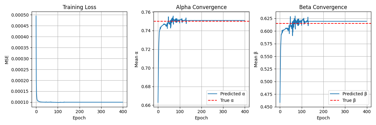
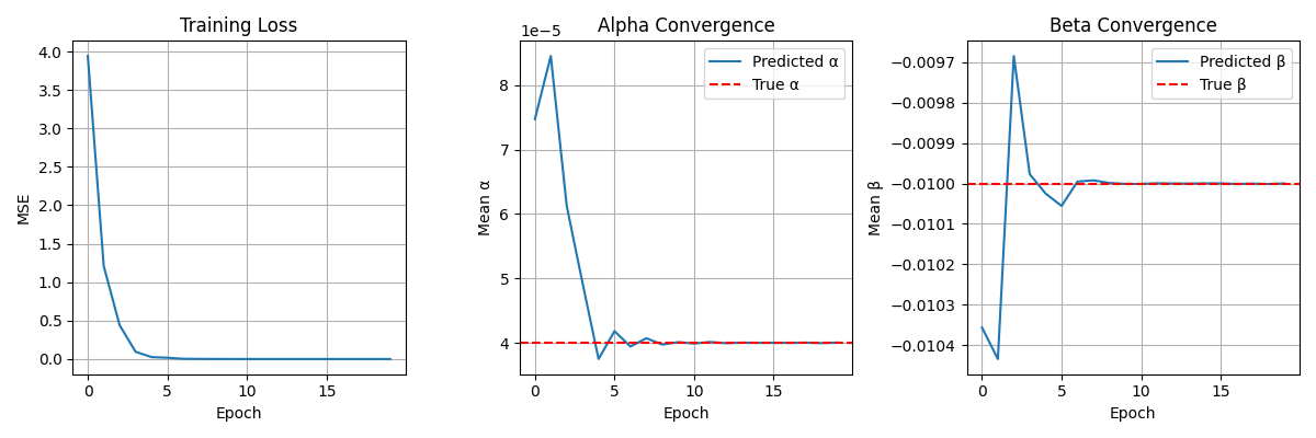
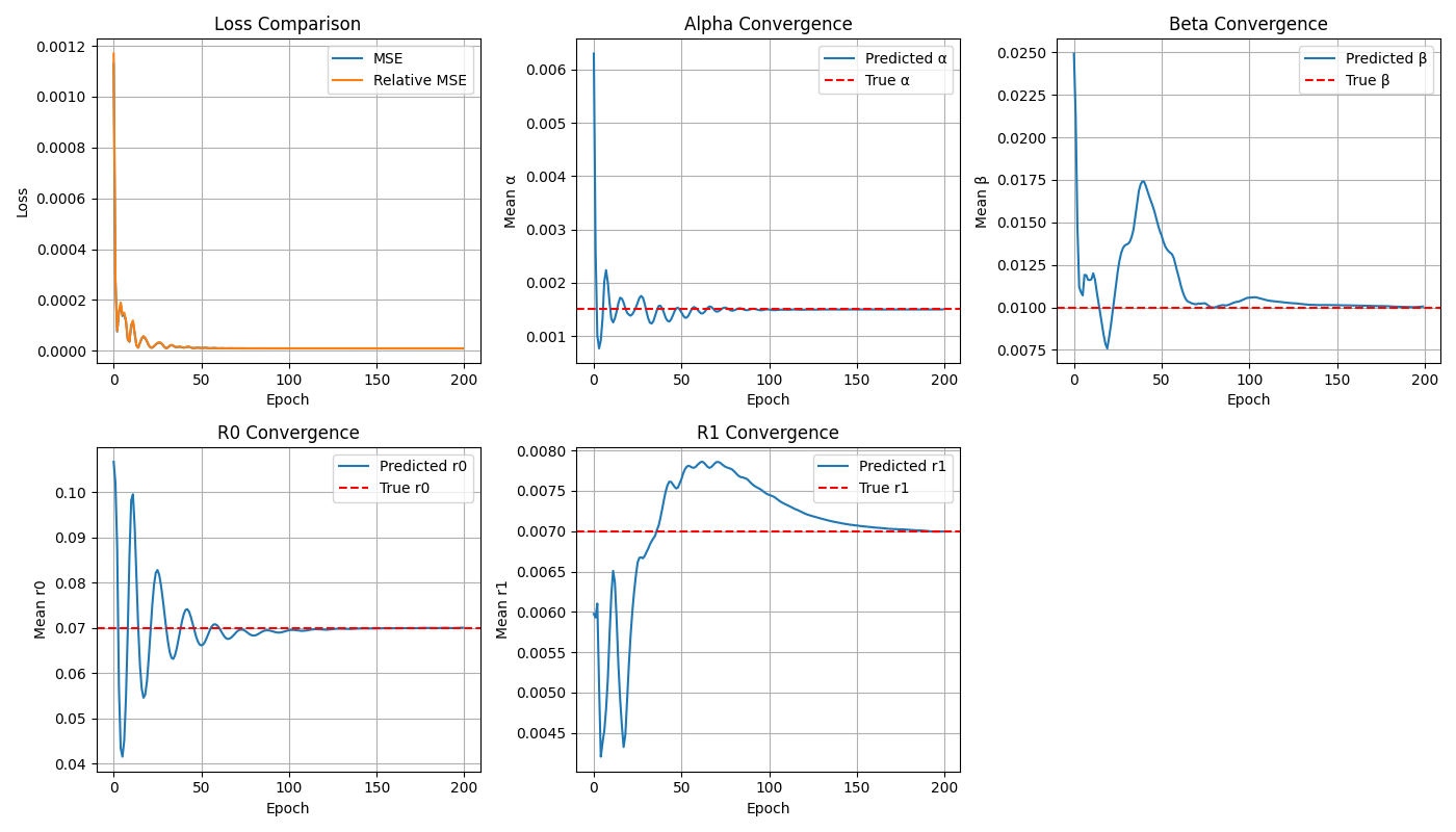
This pipeline leverages mechanistic models and neural ODE–style physics layers (PINNs)
to build physiologically grounded generative modules.
Pipeline B – Inference (Measurement-to-Event, Reverse Information Flow)
Purpose: Infer user states (stress, cognitive load, sleep disruption)
directly from wearable measurements by reversing the information flow of Pipeline A.
Pipeline B does not reconstruct full physiological mechanisms.
Instead, it operates in measurement space. It treats the outputs of
Pipeline A’s Physics Measurement Layer as structured inputs and maps them
directly to event probabilities.
In this architecture, Pipeline A functions as advanced feature engineering.
It transforms raw wearable signals into physiologically meaningful representations,
reducing noise sensitivity and improving interpretability.
Pipeline B then performs robust event inference using these structured features.
Core Components
-
1. Structured Feature Extraction (from Pipeline A)
Rather than relying solely on raw HR or accelerometry, Pipeline B consumes:
- Derived HRV indices (time-domain and frequency-domain)
- Autonomic balance indicators inferred by Pipeline A
- Regime classification (rest vs. movement)
- Signal quality scores
- Temporal stability metrics
These features are physiologically grounded outputs generated by Pipeline A.
-
2. Multi-Scale Temporal Aggregation
Features are computed across multiple time windows (e.g., 30s, 5min, 60min)
to capture both transient responses and sustained deviations.
-
3. Event Inference Model
A supervised or semi-supervised model maps structured features to event probabilities:
- Logistic regression or gradient boosting for interpretable baselines
- Lightweight neural network for nonlinear interactions
- Optional anomaly detection for emerging events
The model outputs calibrated probabilities and confidence scores.
-
4. Uncertainty & Robustness Handling
Pipeline B explicitly accounts for:
- Motion-induced artifacts
- Circadian baseline shifts
- Device-specific noise patterns
This improves generalization in uncontrolled real-world environments.
Relationship Between Pipeline A and Pipeline B
Pipeline B can operate independently using raw features. However,
without Pipeline A, inference relies purely on statistical correlations
and may be vulnerable to confounding and overfitting.
By introducing Pipeline A:
- Signal representations become physiologically interpretable.
- Feature space becomes structured and lower-noise.
- Generalization improves across subjects and devices.
- Event inference becomes explainable rather than purely correlational.
Therefore, Pipeline A provides structured physiological feature engineering,
while Pipeline B provides operational event detection.
Together they form a coherent forward–reverse modeling system.
Conceptual Comparison – Ordinary ML vs Mechanistic-Informed ML
Ordinary ML Pipeline
- Raw Signals
HR, PPG, ACC, etc.
- Basic Preprocessing
Filtering, normalization
- Generic Feature Extraction
Statistical descriptors (mean, variance, FFT, etc.)
- Black-Box ML Model
Learns correlations directly from features
- Predicted State
Stress / Sleep / Cognitive Load
Characteristics: Correlation-driven, limited interpretability, sensitive to noise and distribution shifts.
Mechanistic Model + ML (Proposed)
- Raw Signals
HR, PPG, ACC, etc.
- Physiological Signal Quality & Structuring
Artifact-aware filtering, regime detection
- Mechanistic Feature Synthesis
Autonomic balance proxies, recovery dynamics, response gains
- ML with Physiological Priors
Structured inference constrained by mechanistic meaning
- Predicted State + Interpretation
Event probability with physiological explanation
Characteristics: Physiology-grounded features, improved robustness, enhanced interpretability, better cross-subject generalization.
In the proposed framework, the mechanistic model does not replace machine learning.
Instead, it structures the feature space before learning occurs.
This reduces the hypothesis space the ML model must explore, embeds domain knowledge
into the pipeline, and transforms event detection from pure correlation to
physiology-informed inference.